Examples

Schema Metadata Choices

Structured schema metadata is available directly from the dataclass field metadata through buffalo_panel.config.schema_field_metadata. This example shows how enum-like fields expose machine-readable {"value", "label"} entries that GUI and editor code can consume directly.

Run the example from the repository root with:

uv run python examples/schema_metadata_choices.py

Code:

"""Inspect structured schema metadata choices exposed by Buffalo Panel."""

from __future__ import annotations

from typing import cast

from buffalo_panel.config import (
    PanelCaseSpec,
    SolverSpec,
    schema_field_metadata,
)


def _print_choices(spec_cls: type[object], field_name: str) -> None:
    metadata = schema_field_metadata(spec_cls)[field_name]
    choices = cast(tuple[dict[str, object], ...], metadata.get("choices", ()))
    print(f"{spec_cls.__name__}.{field_name}")
    for choice in choices:
        print(f"  value={choice['value']!r} label={choice['label']!r}")


def main() -> None:
    """Print structured choice metadata for representative schema fields."""
    _print_choices(SolverSpec, "formulation")
    _print_choices(PanelCaseSpec, "schema_version")


if __name__ == "__main__":
    main()

Expected output:

SolverSpec.formulation
  value='hess_smith' label='Hess-Smith'
  value='lumped_vortex' label='Lumped Vortex'
PanelCaseSpec.schema_version
  value=1 label='1'

NACA 0012 Hess-Smith Cases

The structured case schema can be loaded from a YAML file with buffalo_panel.config.load_panel_case and passed to buffalo_panel.config.solve_panel_case. The current wired runtime paths support one embedded Buffalo Wings airfoil body with either the Hess-Smith thick-body formulation or the lumped-vortex thin-body formulation. The two example scripts below demonstrate the Hess-Smith path.

The first is naca0012_designation.py that constructs a NACA 4-digit airfoil from the designation string. Run this example from the repository root with:

uv run python examples/naca0012_designation.py

Input file:

schema_version: 1

units:
  length: m
  angle: deg
  time: s

case:
  name: naca0012_alpha0_designation
  description: >
    Symmetric NACA 0012 airfoil from designation.

solver:
  formulation: hess_smith
  backend: python

freestream:
  speed: 1.0
  alpha: 0.0
  mach: 0.0
  reynolds: 1.0e6

reference:
  speed: 1.0
  length: 1.0
  moment_point: [0.25, 0.0]

geometry:
  bodies:
    - id: airfoil
      airfoil:
        type: naca4
        designation: "0012"
      sampling:
        num_points_per_surface: 41
        spacing: cosine
      placement:
        scale: 1.0
        rotation: 0.0
        rotation_point: [0.0, 0.0]
        translation: [0.0, 0.0]

post:
  surface:
    quantities:
      - tangent_velocity
      - normal_velocity
      - cp
  integrated:
    quantities:
      - cl_pressure
      - cl_circulation
      - cd_pressure
      - cm_pressure

Code:

"""
Solve a Hess-Smith airfoil case with an open trailing edge.

This example uses a designation-based Buffalo Wings NACA 0012 definition,
which currently samples to an open trailing edge in Buffalo Panel's 2D line
geometry. The Hess-Smith open-trailing-edge path:

- Creates a constant strength line source on each panel, where each line source
  has its own strength.
- Creates a constant strength line vortex on each panel, where each line vortex
  shares the same strength.
- Adds one constant strength line source panel and one constant strength line
  vortex panel along the trailing edge gap to close the geometry.
- Relates the closure-panel source and vortex strengths from the body
  trailing-edge source endpoint values.

So along with the Kutta condition, the two relations for the two elements on the
trailing edge gap, and the no penetration surface boundary condition, the system
of unknowns is complete.
"""

from __future__ import annotations

from pathlib import Path

import buffalo_wings.airfoil as bwa

from buffalo_panel.config import load_panel_case, solve_panel_case


def main() -> None:
    """Load the designation-based case and report the open-TE solve path."""
    case_path = Path(__file__).with_name("naca0012_designation.yaml")
    case = load_panel_case(case_path)
    _raw_solution, results = solve_panel_case(case)
    geometry = results.geometry

    print(f"config = {case_path.name}")
    print(f"case = {case.case.name}")
    print("airfoil source = designation")
    print(
        "airfoil: "
        f"{bwa.AirfoilFactory.describe_spec(case.geometry.bodies[0].airfoil).long}"
    )
    print(f"is_closed = {geometry.is_closed}")
    print(f"n_body_panels = {geometry.n_body_panels}")
    print(f"n_panels = {geometry.n_panels}")
    print(f"trailing_edge_panel_index = {geometry.trailing_edge_panel_index}")

    print(f"C_l pressure = {results.integrated.cl_pressure:.6e}")
    print(f"C_l circulation = {results.integrated.cl_circulation:.6e}")
    print(f"C_d pressure = {results.integrated.cd_pressure:.6e}")
    print(f"C_m pressure = {results.integrated.cm_pressure:.6e}")


if __name__ == "__main__":
    main()

Expected output:

config = naca0012_designation.yaml
case = naca0012_alpha0_designation
airfoil source = designation
airfoil: NACA 4-Digit airfoil defined by designation 0012
is_closed = False
n_body_panels = 80
n_panels = 81
trailing_edge_panel_index = 80
C_l pressure = 1.647987e-17
C_l circulation = -1.681278e-17
C_d pressure = -1.967850e-03
C_m pressure = -1.561251e-17

The second is naca0012_parameters.py that constructs a NACA 4-digit airfoil directly from its parameters. Run this example from the repository root with:

uv run python examples/naca0012_parameters.py

Input file:

schema_version: 1

units:
  length: m
  angle: deg
  time: s

case:
  name: naca0012_alpha0_parameters
  description: Symmetric NACA 0012 airfoil from parameters.

solver:
  formulation: hess_smith
  backend: python

freestream:
  speed: 1.0
  alpha: 0.0
  mach: 0.0
  reynolds: 1.0e6

reference:
  speed: 1.0
  length: 1.0
  moment_point: [0.25, 0.0]

geometry:
  bodies:
    - id: airfoil
      airfoil:
        type: naca4
        params:
          m: 0.0
          p: 0.0
          max_thickness: 0.12
          trailing_edge: sharp
          leading_edge_radius: exact
      sampling:
        num_points_per_surface: 41
        spacing: cosine
      placement:
        scale: 1.0
        rotation: 0.0
        rotation_point: [0.0, 0.0]
        translation: [0.0, 0.0]

post:
  surface:
    quantities:
      - tangent_velocity
      - normal_velocity
      - cp
  integrated:
    quantities:
      - cl_pressure
      - cl_circulation
      - cd_pressure
      - cm_pressure

Code:

"""
Solve a Hess-Smith airfoil case with a closed trailing edge.

This example uses a parameters-based Buffalo Wings NACA 0012 definition, which
currently samples to a closed trailing edge in Buffalo Panel's 2D line geometry.
The Hess-Smith closed-trailing-edge path:

- Creates a constant strength line source on each panel, where each line source
  has its own strength.
- Creates a constant strength line vortex on each panel, where each line vortex
  shares the same strength.

So along with the Kutta condition and the no penetration surface boundary
condition, the system of unknowns is complete.
"""

from __future__ import annotations

from pathlib import Path

import buffalo_wings.airfoil as bwa

from buffalo_panel.config import load_panel_case, solve_panel_case


def main() -> None:
    """Solve the configured case and print the main result quantities."""
    case_path = Path(__file__).with_name("naca0012_parameters.yaml")
    case = load_panel_case(case_path)
    _raw_solution, results = solve_panel_case(case)
    geometry = results.geometry

    print(f"file: {case_path.name}")
    print(f"case name: {case.case.name}")
    print(f"case description: {case.case.description}")
    print(
        "airfoil: "
        f"{bwa.AirfoilFactory.describe_spec(case.geometry.bodies[0].airfoil).long}"
    )
    print(f"is_closed = {geometry.is_closed}")
    print(f"n_panels = {geometry.n_body_panels}")
    print(f"n_body_panels = {geometry.n_body_panels}")

    print(f"C_l pressure = {results.integrated.cl_pressure:.6e}")
    print(f"C_l circulation = {results.integrated.cl_circulation:.6e}")
    print(f"C_d pressure = {results.integrated.cd_pressure:.6e}")
    print(f"C_m pressure = {results.integrated.cm_pressure:.6e}")


if __name__ == "__main__":
    main()

Expected output:

file: naca0012_parameters.yaml
case name: naca0012_alpha0_parameters
case description: Symmetric NACA 0012 airfoil from parameters.
airfoil: NACA 4-Digit airfoil defined by explicit params (m=0, p=0, max_thickness=0.12, exact leading edge radius, sharp trailing edge)
is_closed = True
n_panels = 80
n_body_panels = 80
C_l pressure = -9.540979e-18
C_l circulation = 2.711013e-17
C_d pressure = 4.352745e-04
C_m pressure = 3.469447e-18

Element Views

In order to get a better understanding of the influence each element type has on the flow, there are several examples in examples/views.

Point Elements

Representative output for point source:

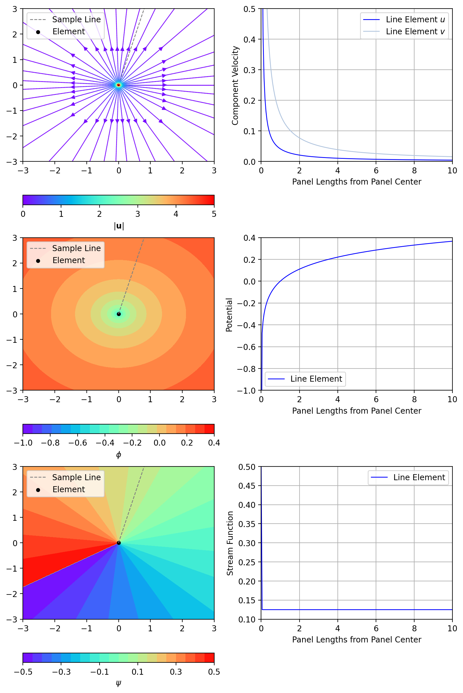
"""Demonstrate the capabilities of a constant strength line source."""

from __future__ import annotations

from collections.abc import Sequence
from pathlib import Path
from typing import cast

import matplotlib.pyplot as plt
import numpy as np
from views_common import (
    create_view,
    equidistant_closed_point,
    parse_args,
    plot_element,
    plot_potential,
    plot_potential_sample,
    plot_ray,
    plot_streamfunction,
    plot_streamfunction_sample,
    plot_streamlines,
    plot_velocity_sample,
    process_output,
)

from buffalo_panel.geometry import ThinBodyLineGeometry2D
from buffalo_panel.views import LineSourcePoint2DView


def main(argv: Sequence[str] | None = None) -> None:
    """Execute main function for example."""
    args = parse_args("point source", argv)

    # Settings for creating view and plots
    theta = np.pi / 6
    r_ray = 10.0
    theta_ray = theta + np.pi / 4

    # Create view
    view = create_view(theta=theta, point=True, view_cls=LineSourcePoint2DView)
    geom = cast(ThinBodyLineGeometry2D, view.geometry)
    x_ray = geom.x_element + np.array(
        [0, r_ray * np.cos(theta_ray)], dtype=np.float64
    )
    y_ray = geom.y_element + np.array(
        [0, r_ray * np.sin(theta_ray)], dtype=np.float64
    )

    # Create figure and suplots
    fig, ax = plt.subplots(  # pyright: ignore[reportUnknownMemberType]
        nrows=3,
        ncols=2,
        figsize=(8, 12),
        constrained_layout=True,
    )
    ax_streamline = ax[0][0]
    ax_velocity_sample = ax[0][1]
    ax_potential = ax[1][0]
    ax_potential_sample = ax[1][1]
    ax_streamfunction = ax[2][0]
    ax_streamfunction_sample = ax[2][1]

    # Plot the streamlines and velocity sample
    x_start, y_start, _ = equidistant_closed_point(
        geom.x_element[0],
        geom.y_element[0],
        0.01,
        40,
    )
    plot_ray(ax_streamline, x_ray, y_ray)
    plot_streamlines(view, fig, ax_streamline, x_start, y_start)
    plot_element(geom, ax_streamline)
    ax_streamline.legend()  # pyright: ignore[reportUnknownMemberType]
    plot_velocity_sample(
        view, None, ax_velocity_sample, r_far=r_ray, theta=theta_ray
    )

    # Plot the potential and sample
    plot_ray(ax_potential, x_ray, y_ray)
    plot_potential(view, fig, ax_potential)
    plot_element(geom, ax_potential)
    ax_potential.legend()  # pyright: ignore[reportUnknownMemberType]
    plot_potential_sample(
        view, None, ax_potential_sample, r_far=r_ray, theta=theta_ray
    )

    # Plot the stream function and sample
    plot_ray(ax_streamfunction, x_ray, y_ray)
    plot_streamfunction(view, fig, ax_streamfunction)
    plot_element(geom, ax_streamfunction)
    ax_streamfunction.legend()  # pyright: ignore[reportUnknownMemberType]
    plot_streamfunction_sample(
        view, None, ax_streamfunction_sample, r_far=r_ray, theta=theta_ray
    )

    process_output(cast(Path, args.output), fig)

    if args.no_show:
        plt.close(fig)
        return

    # Show plot
    plt.show()


if __name__ == "__main__":
    main()

Representative output for point vortex:

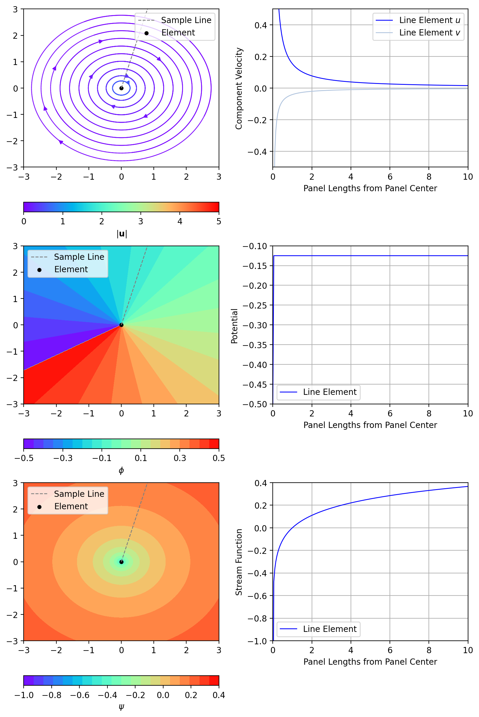
"""Demonstrate the capabilities of a constant strength line vortex."""

from __future__ import annotations

from collections.abc import Sequence
from pathlib import Path
from typing import cast

import matplotlib.pyplot as plt
import numpy as np
from views_common import (
    create_view,
    normal_path,
    parse_args,
    plot_element,
    plot_potential,
    plot_potential_sample,
    plot_ray,
    plot_streamfunction,
    plot_streamfunction_sample,
    plot_streamlines,
    plot_velocity_sample,
    process_output,
)

from buffalo_panel.geometry import ThinBodyLineGeometry2D
from buffalo_panel.views import LineVortexPoint2DView


def main(argv: Sequence[str] | None = None) -> None:
    """Execute main function for example."""
    args = parse_args("point source", argv)

    # Settings for creating view and plots
    theta = np.pi / 6
    r_ray = 10.0
    theta_ray = theta + np.pi / 4

    # Create view
    view = create_view(theta=theta, point=True, view_cls=LineVortexPoint2DView)
    geom = cast(ThinBodyLineGeometry2D, view.geometry)
    x_ray = geom.x_element + np.array(
        [0, r_ray * np.cos(theta_ray)], dtype=np.float64
    )
    y_ray = geom.y_element + np.array(
        [0, r_ray * np.sin(theta_ray)], dtype=np.float64
    )

    # Create figure and suplots
    fig, ax = plt.subplots(  # pyright: ignore[reportUnknownMemberType]
        nrows=3,
        ncols=2,
        figsize=(8, 12),
        constrained_layout=True,
    )
    ax_streamline = ax[0][0]
    ax_velocity_sample = ax[0][1]
    ax_potential = ax[1][0]
    ax_potential_sample = ax[1][1]
    ax_streamfunction = ax[2][0]
    ax_streamfunction_sample = ax[2][1]

    # Plot the streamlines and velocity sample
    x_start, y_start, _ = normal_path(geom.x, geom.y, 0.1, 10)
    plot_ray(ax_streamline, x_ray, y_ray)
    plot_streamlines(view, fig, ax_streamline, x_start, y_start)
    plot_element(geom, ax_streamline)
    ax_streamline.legend()  # pyright: ignore[reportUnknownMemberType]
    plot_velocity_sample(
        view, None, ax_velocity_sample, r_far=r_ray, theta=theta_ray
    )

    # Plot the potential and sample
    plot_ray(ax_potential, x_ray, y_ray)
    plot_potential(view, fig, ax_potential)
    plot_element(geom, ax_potential)
    ax_potential.legend()  # pyright: ignore[reportUnknownMemberType]
    plot_potential_sample(
        view, None, ax_potential_sample, r_far=r_ray, theta=theta_ray
    )

    # Plot the stream function and sample
    plot_ray(ax_streamfunction, x_ray, y_ray)
    plot_streamfunction(view, fig, ax_streamfunction)
    plot_element(geom, ax_streamfunction)
    ax_streamfunction.legend()  # pyright: ignore[reportUnknownMemberType]
    plot_streamfunction_sample(
        view, None, ax_streamfunction_sample, r_far=r_ray, theta=theta_ray
    )

    process_output(cast(Path, args.output), fig)

    if args.no_show:
        plt.close(fig)
        return

    # Show plot
    plt.show()


if __name__ == "__main__":
    main()

Representative output for point doublet:

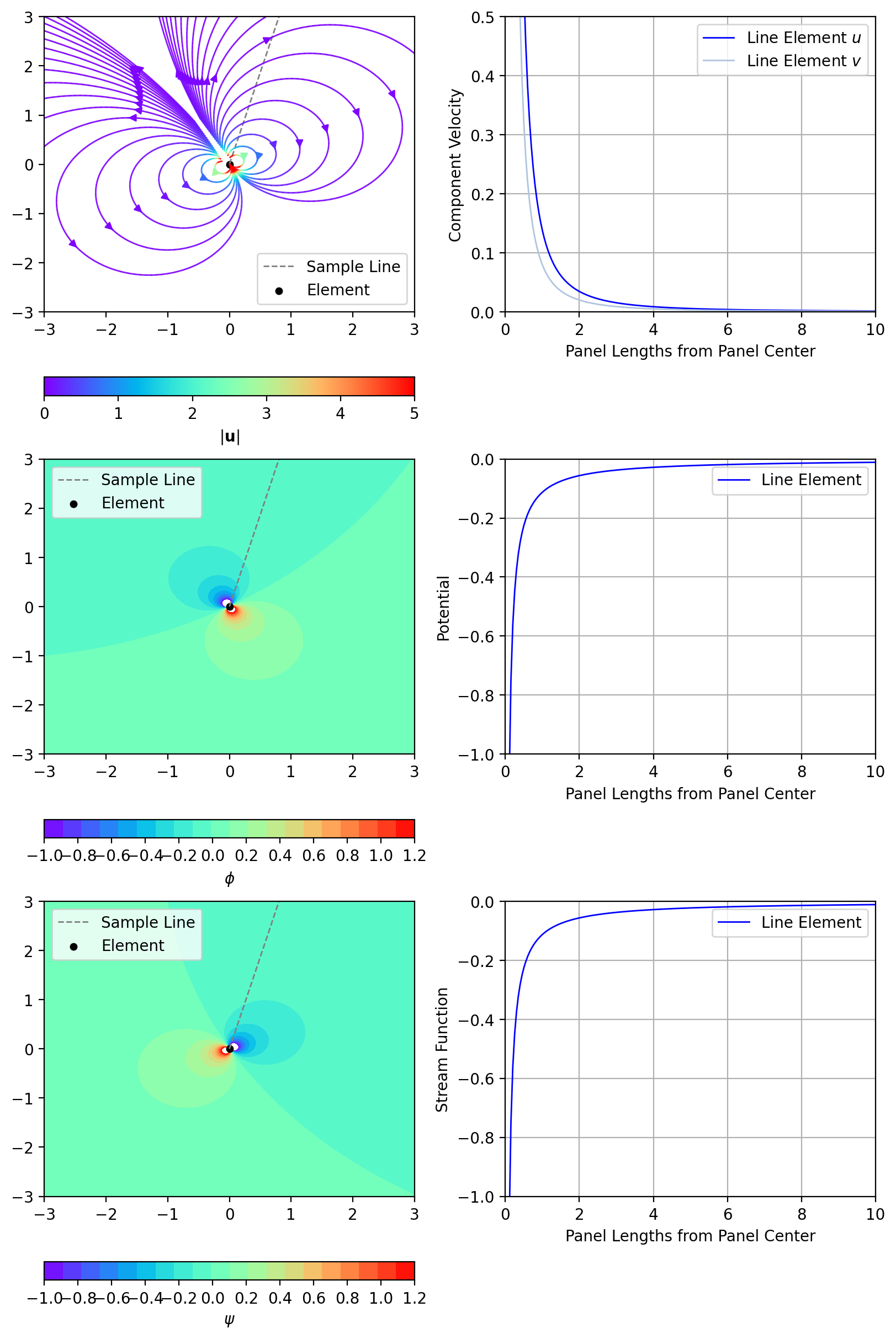
"""Demonstrate the capabilities of a constant strength line doublet."""

from __future__ import annotations

from collections.abc import Sequence
from pathlib import Path
from typing import cast

import matplotlib.pyplot as plt
import numpy as np
from views_common import (
    create_view,
    equidistant_closed_line_path,
    parse_args,
    plot_element,
    plot_potential,
    plot_potential_sample,
    plot_ray,
    plot_streamfunction,
    plot_streamfunction_sample,
    plot_streamlines,
    plot_velocity_sample,
    process_output,
)

from buffalo_panel.geometry import ThinBodyLineGeometry2D
from buffalo_panel.views import LineDoubletPoint2DView


def main(argv: Sequence[str] | None = None) -> None:
    """Execute main function for example."""
    args = parse_args("point source", argv)

    # Settings for creating view and plots
    theta = np.pi / 6
    r_ray = 10.0
    theta_ray = theta + np.pi / 4

    # Create view
    view = create_view(theta=theta, point=True, view_cls=LineDoubletPoint2DView)
    geom = cast(ThinBodyLineGeometry2D, view.geometry)
    x_ray = geom.x_element + np.array(
        [0, r_ray * np.cos(theta_ray)], dtype=np.float64
    )
    y_ray = geom.y_element + np.array(
        [0, r_ray * np.sin(theta_ray)], dtype=np.float64
    )

    # Create figure and suplots
    fig, ax = plt.subplots(  # pyright: ignore[reportUnknownMemberType]
        nrows=3,
        ncols=2,
        figsize=(8, 12),
        constrained_layout=True,
    )
    ax_streamline = ax[0][0]
    ax_velocity_sample = ax[0][1]
    ax_potential = ax[1][0]
    ax_potential_sample = ax[1][1]
    ax_streamfunction = ax[2][0]
    ax_streamfunction_sample = ax[2][1]

    # Plot the streamlines and velocity sample
    x_start, y_start, _ = equidistant_closed_line_path(geom.x, geom.y, 0.01, 40)
    x_start_1 = 0.05 * np.cos(theta) - np.linspace(0.1, 1, 20) * np.sin(theta)
    y_start_1 = 0.05 * np.sin(theta) + np.linspace(0.1, 1, 20) * np.cos(theta)
    x_start_2 = -0.05 * np.cos(theta) - np.linspace(0.1, 1, 20) * np.sin(theta)
    y_start_2 = -0.05 * np.sin(theta) + np.linspace(0.1, 1, 20) * np.cos(theta)
    x_start = np.concatenate([x_start_1, x_start_2])
    y_start = np.concatenate([y_start_1, y_start_2])
    plot_ray(ax_streamline, x_ray, y_ray)
    plot_streamlines(view, fig, ax_streamline, x_start, y_start)
    plot_element(geom, ax_streamline)
    ax_streamline.legend()  # pyright: ignore[reportUnknownMemberType]
    plot_velocity_sample(
        view, None, ax_velocity_sample, r_far=r_ray, theta=theta_ray
    )

    # Plot the potential and sample
    plot_ray(ax_potential, x_ray, y_ray)
    plot_potential(view, fig, ax_potential)
    plot_element(geom, ax_potential)
    ax_potential.legend()  # pyright: ignore[reportUnknownMemberType]
    plot_potential_sample(
        view, None, ax_potential_sample, r_far=r_ray, theta=theta_ray
    )

    # Plot the stream function and sample
    plot_ray(ax_streamfunction, x_ray, y_ray)
    plot_streamfunction(view, fig, ax_streamfunction)
    plot_element(geom, ax_streamfunction)
    ax_streamfunction.legend()  # pyright: ignore[reportUnknownMemberType]
    plot_streamfunction_sample(
        view, None, ax_streamfunction_sample, r_far=r_ray, theta=theta_ray
    )

    process_output(cast(Path, args.output), fig)

    if args.no_show:
        plt.close(fig)
        return

    # Show plot
    plt.show()


if __name__ == "__main__":
    main()

Constant Strength Line Elements

Representative output for constant strength line source and equivalent point source:

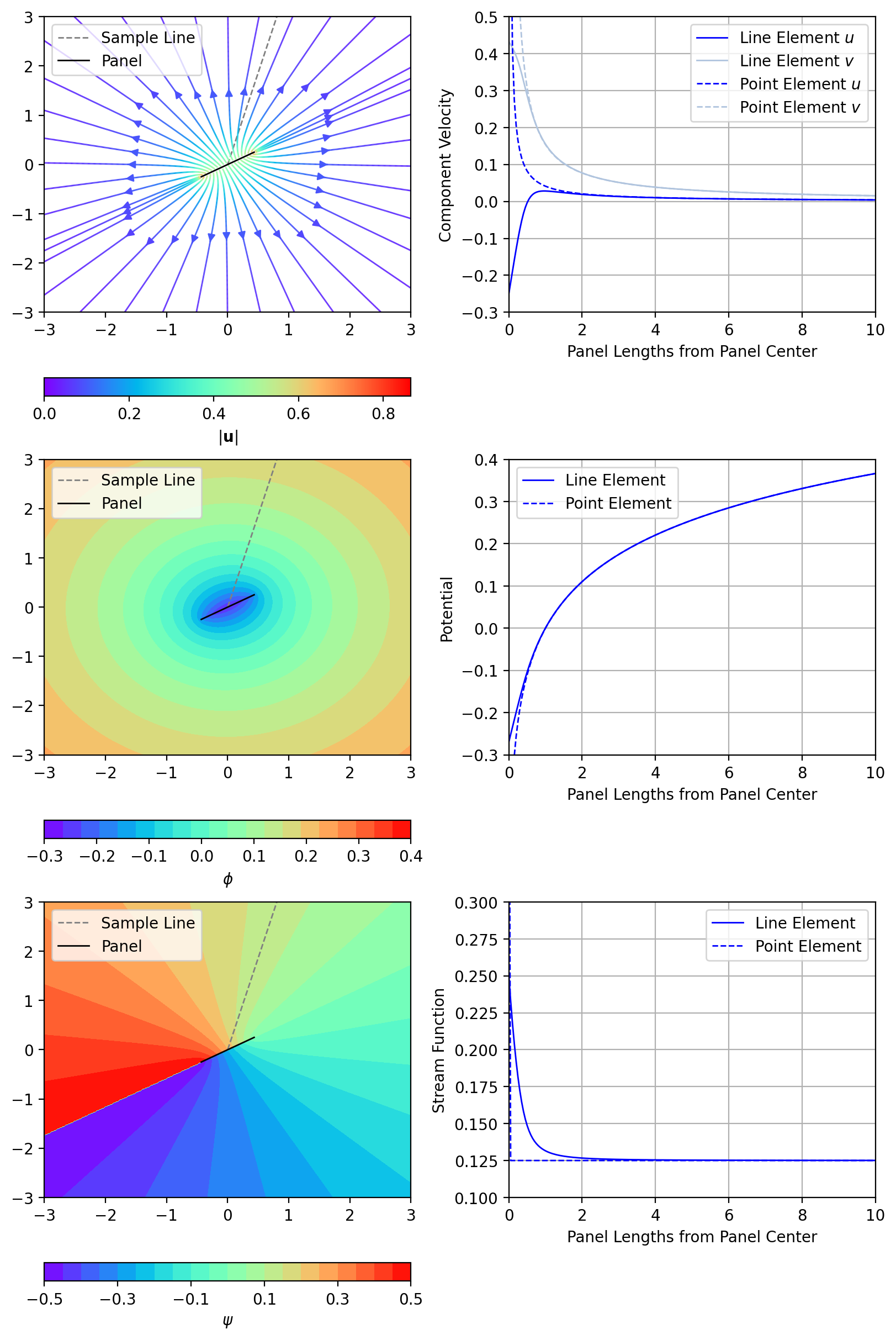
"""Demonstrate the capabilities of a constant strength line source."""

from __future__ import annotations

from collections.abc import Sequence
from pathlib import Path
from typing import cast

import matplotlib.pyplot as plt
import numpy as np
from views_common import (
    create_view,
    equidistant_closed_line_path,
    parse_args,
    plot_panel,
    plot_potential,
    plot_potential_sample,
    plot_ray,
    plot_streamfunction,
    plot_streamfunction_sample,
    plot_streamlines,
    plot_velocity_sample,
    process_output,
)

from buffalo_panel.geometry import ThinBodyLineGeometry2D
from buffalo_panel.views import LineSourceConstant2DView, LineSourcePoint2DView


def main(argv: Sequence[str] | None = None) -> None:
    """Execute main function for example."""
    args = parse_args("point source", argv)

    # Settings for creating view and plots
    theta = np.pi / 6
    r_ray = 10.0
    theta_ray = theta + np.pi / 4

    # Create view
    view = create_view(
        theta=theta, point=False, view_cls=LineSourceConstant2DView
    )
    geom = cast(ThinBodyLineGeometry2D, view.geometry)
    x_ray = geom.x_col[0] + [0, r_ray * np.cos(theta_ray)]
    y_ray = geom.y_col[0] + [0, r_ray * np.sin(theta_ray)]
    point_view = create_view(
        theta=theta, point=True, view_cls=LineSourcePoint2DView
    )

    # Create figure and suplots
    fig, ax = plt.subplots(  # pyright: ignore[reportUnknownMemberType]
        nrows=3,
        ncols=2,
        figsize=(8, 12),
        constrained_layout=True,
    )
    ax_streamline = ax[0][0]
    ax_velocity_sample = ax[0][1]
    ax_potential = ax[1][0]
    ax_potential_sample = ax[1][1]
    ax_streamfunction = ax[2][0]
    ax_streamfunction_sample = ax[2][1]

    # Plot the streamlines and velocity sample
    x_start, y_start, _ = equidistant_closed_line_path(geom.x, geom.y, 0.01, 40)
    plot_ray(ax_streamline, x_ray, y_ray)
    plot_streamlines(view, fig, ax_streamline, x_start, y_start)
    plot_panel(geom, ax_streamline)
    ax_streamline.legend()  # pyright: ignore[reportUnknownMemberType]
    plot_velocity_sample(
        view, point_view, ax_velocity_sample, r_far=r_ray, theta=theta_ray
    )

    # Plot the potential and sample
    plot_ray(ax_potential, x_ray, y_ray)
    plot_potential(view, fig, ax_potential)
    plot_panel(geom, ax_potential)
    ax_potential.legend()  # pyright: ignore[reportUnknownMemberType]
    plot_potential_sample(
        view, point_view, ax_potential_sample, r_far=r_ray, theta=theta_ray
    )

    # Plot the stream function and sample
    plot_ray(ax_streamfunction, x_ray, y_ray)
    plot_streamfunction(view, fig, ax_streamfunction)
    plot_panel(geom, ax_streamfunction)
    ax_streamfunction.legend()  # pyright: ignore[reportUnknownMemberType]
    plot_streamfunction_sample(
        view, point_view, ax_streamfunction_sample, r_far=r_ray, theta=theta_ray
    )

    process_output(cast(Path, args.output), fig)

    if args.no_show:
        plt.close(fig)
        return

    # Show plot
    plt.show()


if __name__ == "__main__":
    main()

Representative output for constant strength line vortex and equivalent point vortex:

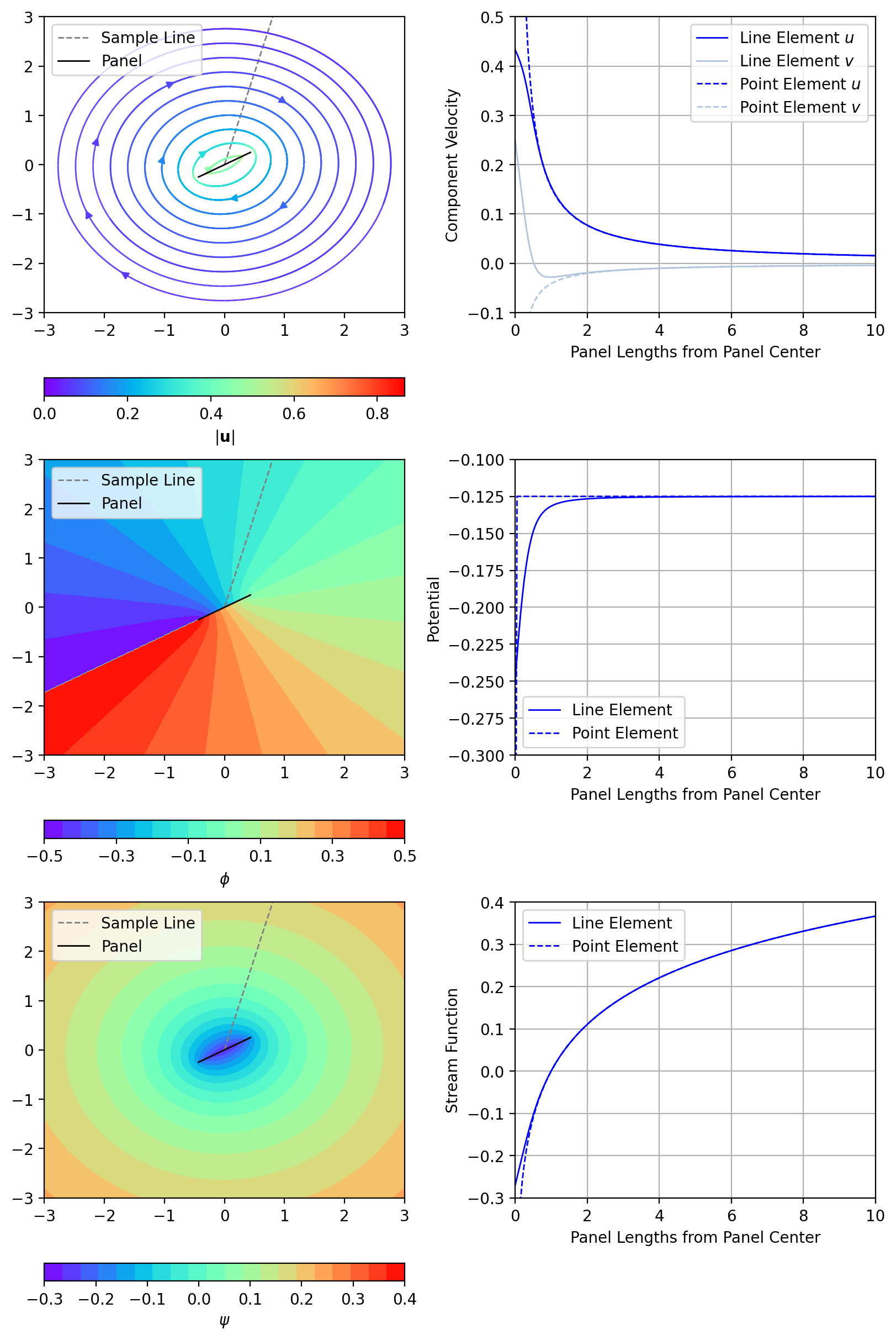
"""Demonstrate the capabilities of a constant strength line source."""

from __future__ import annotations

from collections.abc import Sequence
from pathlib import Path
from typing import cast

import matplotlib.pyplot as plt
import numpy as np
from views_common import (
    create_view,
    normal_path,
    parse_args,
    plot_panel,
    plot_potential,
    plot_potential_sample,
    plot_ray,
    plot_streamfunction,
    plot_streamfunction_sample,
    plot_streamlines,
    plot_velocity_sample,
    process_output,
)

from buffalo_panel.geometry import ThinBodyLineGeometry2D
from buffalo_panel.views import LineVortexConstant2DView, LineVortexPoint2DView


def main(argv: Sequence[str] | None = None) -> None:
    """Execute main function for example."""
    args = parse_args("point source", argv)

    # Settings for creating view and plots
    theta = np.pi / 6
    r_ray = 10.0
    theta_ray = theta + np.pi / 4

    # Create view
    view = create_view(
        theta=theta, point=False, view_cls=LineVortexConstant2DView
    )
    geom = cast(ThinBodyLineGeometry2D, view.geometry)
    x_ray = geom.x_col[0] + [0, r_ray * np.cos(theta_ray)]
    y_ray = geom.y_col[0] + [0, r_ray * np.sin(theta_ray)]
    point_view = create_view(
        theta=theta, point=True, view_cls=LineVortexPoint2DView
    )

    # Create figure and suplots
    fig, ax = plt.subplots(  # pyright: ignore[reportUnknownMemberType]
        nrows=3,
        ncols=2,
        figsize=(8, 12),
        constrained_layout=True,
    )
    ax_streamline = ax[0][0]
    ax_velocity_sample = ax[0][1]
    ax_potential = ax[1][0]
    ax_potential_sample = ax[1][1]
    ax_streamfunction = ax[2][0]
    ax_streamfunction_sample = ax[2][1]

    # Plot the streamlines and velocity sample
    x_start, y_start, _ = normal_path(geom.x, geom.y, 0.1, 10)
    plot_ray(ax_streamline, x_ray, y_ray)
    plot_streamlines(view, fig, ax_streamline, x_start, y_start)
    plot_panel(geom, ax_streamline)
    ax_streamline.legend()  # pyright: ignore[reportUnknownMemberType]
    plot_velocity_sample(
        view, point_view, ax_velocity_sample, r_far=r_ray, theta=theta_ray
    )

    # Plot the potential and sample
    plot_ray(ax_potential, x_ray, y_ray)
    plot_potential(view, fig, ax_potential)
    plot_panel(geom, ax_potential)
    ax_potential.legend()  # pyright: ignore[reportUnknownMemberType]
    plot_potential_sample(
        view, point_view, ax_potential_sample, r_far=r_ray, theta=theta_ray
    )

    # Plot the stream function and sample
    plot_ray(ax_streamfunction, x_ray, y_ray)
    plot_streamfunction(view, fig, ax_streamfunction)
    plot_panel(geom, ax_streamfunction)
    ax_streamfunction.legend()  # pyright: ignore[reportUnknownMemberType]
    plot_streamfunction_sample(
        view, point_view, ax_streamfunction_sample, r_far=r_ray, theta=theta_ray
    )

    process_output(cast(Path, args.output), fig)

    if args.no_show:
        plt.close(fig)
        return

    # Show plot
    plt.show()


if __name__ == "__main__":
    main()

Representative output for constant strength line doublet and equivalent point dobulet:

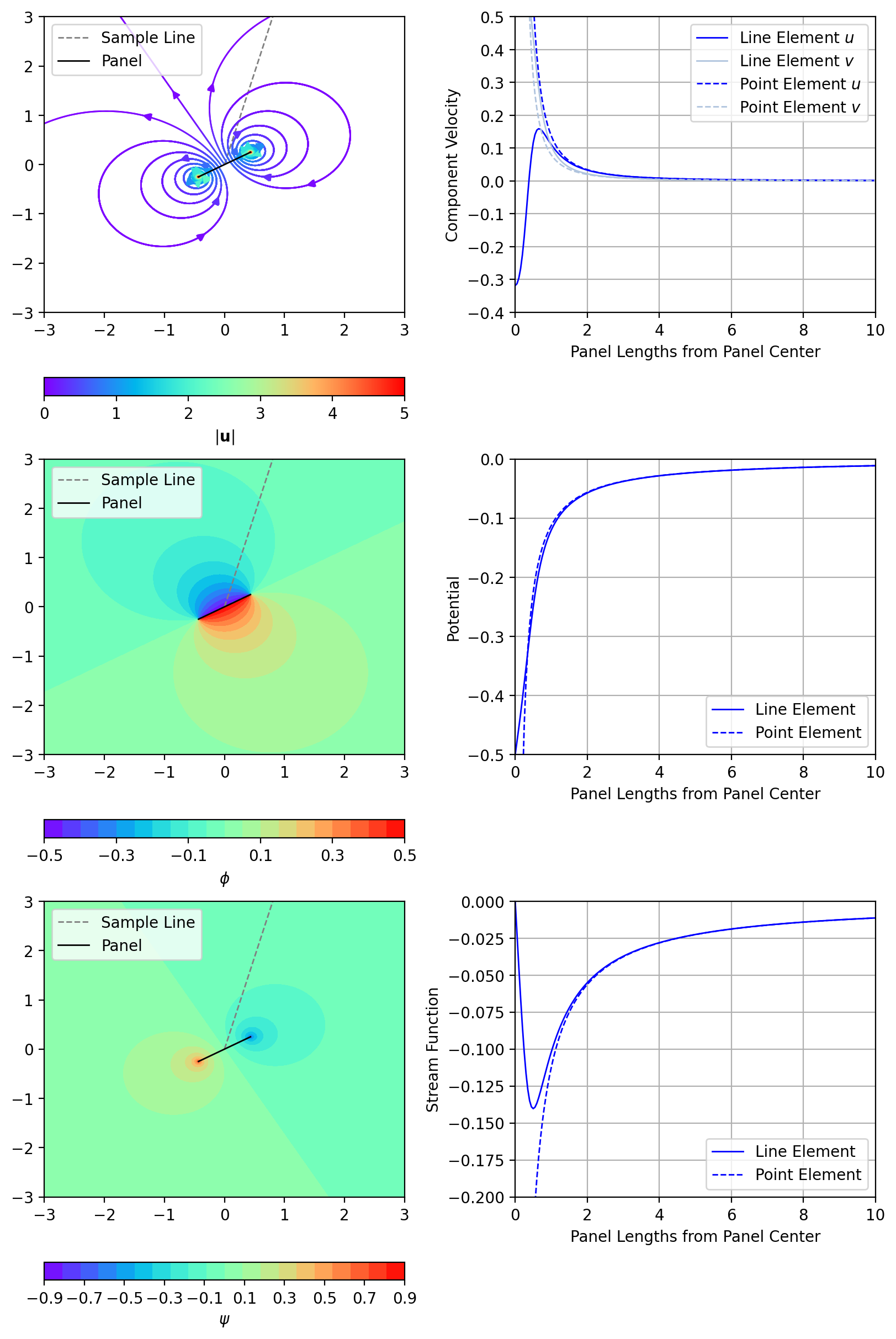
"""Demonstrate the capabilities of a constant strength line source."""

from __future__ import annotations

from collections.abc import Sequence
from pathlib import Path
from typing import cast

import matplotlib.pyplot as plt
import numpy as np
from views_common import (
    create_view,
    equidistant_closed_line_path,
    parse_args,
    plot_panel,
    plot_potential,
    plot_potential_sample,
    plot_ray,
    plot_streamfunction,
    plot_streamfunction_sample,
    plot_streamlines,
    plot_velocity_sample,
    process_output,
)

from buffalo_panel.geometry import ThinBodyLineGeometry2D
from buffalo_panel.views import (
    LineDoubletConstant2DView,
    LineDoubletPoint2DView,
)


def main(argv: Sequence[str] | None = None) -> None:
    """Execute main function for example."""
    args = parse_args("point source", argv)

    # Settings for creating view and plots
    theta = np.pi / 6
    r_ray = 10.0
    theta_ray = theta + np.pi / 4

    # Create view
    view = create_view(
        theta=theta, point=False, view_cls=LineDoubletConstant2DView
    )
    geom = cast(ThinBodyLineGeometry2D, view.geometry)
    x_ray = geom.x_col[0] + [0, r_ray * np.cos(theta_ray)]
    y_ray = geom.y_col[0] + [0, r_ray * np.sin(theta_ray)]
    point_view = create_view(
        theta=theta, point=True, view_cls=LineDoubletPoint2DView
    )

    # Create figure and suplots
    fig, ax = plt.subplots(  # pyright: ignore[reportUnknownMemberType]
        nrows=3,
        ncols=2,
        figsize=(8, 12),
        constrained_layout=True,
    )
    ax_streamline = ax[0][0]
    ax_velocity_sample = ax[0][1]
    ax_potential = ax[1][0]
    ax_potential_sample = ax[1][1]
    ax_streamfunction = ax[2][0]
    ax_streamfunction_sample = ax[2][1]

    # Plot the streamlines and velocity sample
    x_start, y_start, _ = equidistant_closed_line_path(geom.x, geom.y, 0.01, 40)
    plot_ray(ax_streamline, x_ray, y_ray)
    plot_streamlines(view, fig, ax_streamline, x_start, y_start)
    plot_panel(geom, ax_streamline)
    ax_streamline.legend()  # pyright: ignore[reportUnknownMemberType]
    plot_velocity_sample(
        view, point_view, ax_velocity_sample, r_far=r_ray, theta=theta_ray
    )

    # Plot the potential and sample
    plot_ray(ax_potential, x_ray, y_ray)
    plot_potential(view, fig, ax_potential)
    plot_panel(geom, ax_potential)
    ax_potential.legend()  # pyright: ignore[reportUnknownMemberType]
    plot_potential_sample(
        view, point_view, ax_potential_sample, r_far=r_ray, theta=theta_ray
    )

    # Plot the stream function and sample
    plot_ray(ax_streamfunction, x_ray, y_ray)
    plot_streamfunction(view, fig, ax_streamfunction)
    plot_panel(geom, ax_streamfunction)
    ax_streamfunction.legend()  # pyright: ignore[reportUnknownMemberType]
    plot_streamfunction_sample(
        view, point_view, ax_streamfunction_sample, r_far=r_ray, theta=theta_ray
    )

    process_output(cast(Path, args.output), fig)

    if args.no_show:
        plt.close(fig)
        return

    # Show plot
    plt.show()


if __name__ == "__main__":
    main()